Building a Logistic Regression Classifier in PyTorch

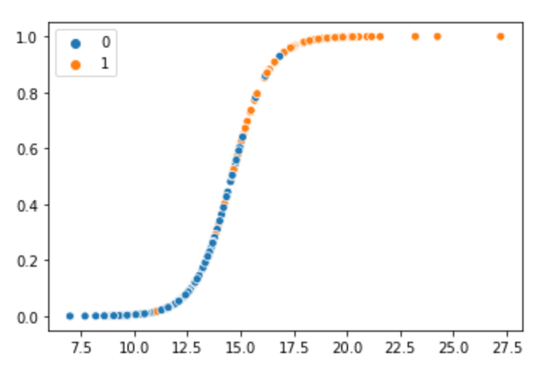
Logistic regression is a popular machine learning algorithm used for binary classification problems. It models the probability of an input belonging to a particular class. In this post, we will walk through how to implement logistic regression in PyTorch. While there are many other libraries such as sklearn which provide logistic regression classifiers out of the box, it is quite useful to understand to how to write a logistic regression using PyTorch.

Importing PyTorch

First, we import PyTorch:

import torch
import torch.nn as nn
from torch.utils.data import Dataset, DataLoader

This gives us access to the core PyTorch library, nn module for neural networks, and DataLoader for easy data loading.

Defining the Model

Next, we define our logistic regression model by subclassing nn.Module:

class LogisticRegression(nn.Module):
    def __init__(self, input_dim, output_dim):
        super(LogisticRegression, self).__init__()
        self.linear = nn.Linear(input_dim, output_dim)
        
    def forward(self, x):
        out = self.linear(x)
        return torch.sigmoid(out)

Our model takes an input tensor x and passes it through a single linear layer to get logits. We then apply sigmoid to get probability outputs between 0-1.

Here is an example of how to load a CSV file in PyTorch

from torch.utils.data import Dataset, DataLoader
from sklearn.datasets import load_boston
import pandas as pd
import numpy as np

class BostonHousingDataset(Dataset):
    def __init__(self):
        boston = load_boston()
        df = pd.DataFrame(boston.data, columns=boston.feature_names)
        df['MEDV'] = boston.target
        self.data = torch.tensor(df.values, dtype=torch.float32)

    def __len__(self):
        return len(self.data)

    def __getitem__(self, index):
        features = self.data[index, :-1]
        target = self.data[index, -1]
        return features, target

# Create a Dataset from the Boston Housing data
dataset = BostonHousingDataset()

# Create a DataLoader
dataloader = DataLoader(dataset, batch_size=32, shuffle=True)

# Iterate over the data
for i, (inputs, labels) in enumerate(dataloader):
    # Assuming you have a model and loss function
    # outputs = model(inputs)
    # loss = loss_fn(outputs, labels)
    print(f'Batch {i+1}')
    print('Inputs:', inputs)
    print('Labels:', labels)
    print()

Preparing Data

We can use PyTorch's DataLoader class to easily load data batches:

# Define dataset
class MyDataset(Dataset):
  ...

# Create data loader 
train_loader = DataLoader(MyDataset(), batch_size=32, shuffle=True)

Our custom Dataset class should implement __len__ and __getitem__ to load data examples.

Training the Model

We train our model by iterating through data batches:

criterion = nn.BCELoss()
optimizer = torch.optim.SGD(model.parameters(), lr=0.01) 

for epoch in range(num_epochs):
  for i, (x, y) in enumerate(train_loader):
    # Forward pass
    y_pred = model(x) 
    
    # Compute loss
    loss = criterion(y_pred, y)
    
    # Backward pass
    loss.backward()
    
    # Update parameters
    optimizer.step()
    
    # Reset gradients
    optimizer.zero_grad() 

We use binary cross-entropy loss and stochastic gradient descent to update parameters. This allows our model to learn from data.

Evaluating Results

Finally, we can test our model on an evaluation set:

y_pred = model(x_test)
acc = torch.sum(y_pred.round() == y_test)/len(y_test)
print('Accuracy:', acc.item())

This allows us to quantify the performance of our logistic regression classifier.

Some other metrics which are typically used for evaluating model performance

1. Accuracy: Measures the proportion of correct predictions in the total sample.
2. Precision: Measures how many of the items identified as positive are actually positive.
3. Recall: Measures how many of the actual positive cases were identified correctly.
4. F1-Score: Harmonic mean of Precision and Recall.
5. ROC-AUC: The area under the Receiver Operating Characteristic curve.
6. Confusion Matrix: A table used to describe the performance of a classification model.

We can compute those metrics by using the following code

from sklearn.metrics import precision_score, recall_score, f1_score, roc_auc_score, confusion_matrix
import matplotlib.pyplot as plt
from sklearn.metrics import roc_curve


# Assuming y_pred and y_test are PyTorch tensors, and model has already been trained
y_pred_np = y_pred.detach().numpy().round()
y_test_np = y_test.detach().numpy()


# Precision
precision = precision_score(y_test_np, y_pred_np)
print(f'Precision: {precision}')

# Recall
recall = recall_score(y_test_np, y_pred_np)
print(f'Recall: {recall}')

# F1-Score
f1 = f1_score(y_test_np, y_pred_np)
print(f'F1 Score: {f1}')

# ROC-AUC
roc_auc = roc_auc_score(y_test_np, y_pred_np)
print(f'ROC AUC: {roc_auc}')

# Confusion Matrix
conf_mat = confusion_matrix(y_test_np, y_pred_np)
print(f'Confusion Matrix: \n{conf_mat}')

# ROC Curve
fpr, tpr, thresholds = roc_curve(y_test_np, y_pred_np)
plt.plot(fpr, tpr)
plt.title('ROC Curve')
plt.xlabel('False Positive Rate')
plt.ylabel('True Positive Rate')
plt.show()

In this post, we implemented logistic regression for binary classification in PyTorch by defining a model, training on data batches, and evaluating results. PyTorch provides a flexible framework for quickly building and training neural networks.

Challenges with Logistic Regression

While logistic regressions can build good machine learning models, there are some challenges with logistic regression models.

1. Assumption of linearity: Logistic regression assumes that the relationship between the independent variables and the log odds of the dependent variable is linear. If this assumption is violated, the model's predictions may be inaccurate.
2. Multicollinearity: Logistic regression is sensitive to multicollinearity, which occurs when independent variables are highly correlated with each other. Multicollinearity can lead to unstable estimates of the regression coefficients and make it difficult to interpret the results.
3. Overfitting: Overfitting occurs when the model is too complex and fits the training data too closely, resulting in poor performance on new, unseen data. Logistic regression can be prone to overfitting, especially when there are many independent variables and a limited number of observations.
4. Heteroscedasticity: Heteroscedasticity occurs when the variance of the errors is not constant across all levels of the independent variables. Logistic regression assumes homoscedasticity, which can lead to biased estimates of the regression coefficients.
5. Outliers: Logistic regression is sensitive to outliers, which can have a significant impact on the model's predictions. Outliers can occur due to errors in data collection or measurement, or they may represent rare but important cases.
6. Non-linear relationships: Logistic regression assumes a linear relationship between the independent variables and the log odds of the dependent variable. However, in some cases, the relationship may be non-linear, which can lead to inaccurate predictions.
7. High-dimensional data: Logistic regression can be computationally expensive and may not perform well when there are many independent variables relative to the number of observations. This is known as the "curse of dimensionality."