Transformer Architecture with Examples
Let’s dive into the Transformer architecture and break down the dimensions of the input, input embeddings, and how data transforms through the model. I’ll provide a clear, detailed explanation of the full architecture, focusing on how the input evolves step-by-step. Since you’re asking about dimensions and transformations, I’ll assume you’re familiar with the basics but want a precise, end-to-end walkthrough.
Transformer Architecture Overview
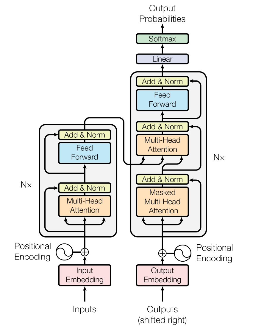
The Transformer, introduced in "Attention is All You Need" (Vaswani et al., 2017), consists of an encoder and a decoder, both built from stacked layers. It’s designed for sequence-to-sequence tasks (e.g., translation), but I’ll describe the general architecture, noting dimensions at each step. For concreteness, I’ll use typical values like a model dimension ( d_{\text{model}} = 512 ) and a vocabulary size ( V = 30,000 ), though these can vary (e.g., BERT uses ( d_{\text{model}} = 768 ), GPT varies by size).
Step 1: Input
- Raw Input: A sequence of tokens (words, subwords, etc.) from a vocabulary. For example, a sentence like "The cat sleeps" might be tokenized into (["The", "cat", "sleeps"]).
- Dimensions: If the input sequence has length ( T ) (e.g., ( T = 3 ) for "The cat sleeps"), the input is a 1D tensor of token IDs:
- Shape: ( [T] ), e.g., ( [784, 231, 1509] ) (token IDs from the vocabulary).
- Batch Consideration: In practice, we process batches. For batch size ( B ), the input becomes:
- Shape: ( [B, T] ).
Step 2: Input Embeddings
- Transformation: Each token ID is mapped to a dense vector using an embedding layer (a lookup table).
- Embedding Matrix: A learnable matrix of shape ( [V, d_{\text{model}}] ), where ( V ) is the vocabulary size (e.g., 30,000) and ( d_{\text{model}} ) is the embedding dimension (e.g., 512).
- Output: Each token ID is replaced by its corresponding ( d_{\text{model}} )-dimensional vector.
- Dimensions: For a single sequence, the output is:
- Shape: ( [T, d_{\text{model}}] ), e.g., ( [3, 512] ).
- For a batch: ( [B, T, d_{\text{model}}] ), e.g., ( [B, 3, 512] ).
- Example: "The" (ID 784) → ( [0.1, -0.3, ..., 0.5] ) (a 512D vector).
Step 3: Positional Encodings
- Why: Transformers lack recurrence, so they need positional information to understand token order.
- Transformation: Add fixed or learned positional encodings to the input embeddings. These are vectors of the same size as the embeddings (( d_{\text{model}} )).
- Formula (fixed, sinusoidal):
- ( PE(pos, 2i) = \sin(pos / 10000^{2i / d_{\text{model}}}) )
- ( PE(pos, 2i+1) = \cos(pos / 10000^{2i / d_{\text{model}}}) )
- Where ( pos ) is the position (0 to ( T-1 )), and ( i ) is the dimension index (0 to ( d_{\text{model}}/2 - 1 )).
- Output: Input embeddings + positional encodings.
- Dimensions: Unchanged, still ( [B, T, d_{\text{model}}] ).
Step 4: Encoder
The encoder has ( N ) identical layers (e.g., ( N = 6 )). Each layer has two main sub-layers:
a) Multi-Head Self-Attention
- Inputs: ( [B, T, d_{\text{model}}] ) (e.g., ( [B, 3, 512] )).
- Mechanism: Compute queries (( Q )), keys (( K )), and values (( V )) using linear projections:
- ( Q = X W_Q ), ( K = X W_K ), ( V = X W_V ), where ( X ) is the input, and each ( W ) is ( [d_{\text{model}}, d_k] ) or ( [d_{\text{model}}, d_v] ).
- Typically, ( d_k = d_v = d_{\text{model}} / h ), where ( h ) is the number of heads (e.g., ( h = 8 ), so ( d_k = d_v = 64 )).
- Attention: ( \text{Attention}(Q, K, V) = \text{softmax}(QK^T / \sqrt{d_k}) V ).
- ( QK^T ): ( [B, T, T] ) per head.
- Output per head: ( [B, T, d_v] ).
- Multi-Head: Concatenate ( h ) heads, then project with ( W_O ) (( [h \cdot d_v, d_{\text{model}}] )):
- Output: ( [B, T, d_{\text{model}}] ).
- Residual + Norm: Add input to output, then layer normalize.
b) Feed-Forward Network (FFN)
- Inputs: ( [B, T, d_{\text{model}}] ).
- Transformation: Per token, apply two linear layers with a ReLU:
- ( FFN(x) = \max(0, x W_1 + b_1) W_2 + b_2 ).
- ( W_1 ): ( [d_{\text{model}}, d_{\text{ff}}] ) (e.g., ( d_{\text{ff}} = 2048 )).
- ( W_2 ): ( [d_{\text{ff}}, d_{\text{model}}] ).
- Output: ( [B, T, d_{\text{model}}] ).
- Residual + Norm: Add input, then normalize.
- Encoder Output: After ( N ) layers, still ( [B, T, d_{\text{model}}] ).
Step 5: Decoder
The decoder also has ( N ) layers, with three sub-layers per layer. It generates the output sequence (length ( T' )) autoregressively.
a) Masked Multi-Head Self-Attention
- Inputs: Output embeddings (shifted right) + positional encodings, shape ( [B, T', d_{\text{model}}] ).
- Masking: Prevent attending to future tokens using a causal mask.
- Output: ( [B, T', d_{\text{model}}] ).
b) Multi-Head Attention (Encoder-Decoder)
- Inputs: Decoder’s ( Q ) (( [B, T', d_{\text{model}}] )), encoder’s ( K ) and ( V ) (( [B, T, d_{\text{model}}] )).
- Output: ( [B, T', d_{\text{model}}] ).
c) Feed-Forward Network
- Same as encoder: ( [B, T', d_{\text{model}}] ).
- Decoder Output: After ( N ) layers, ( [B, T', d_{\text{model}}] ).
Step 6: Output Projection
- Transformation: Linear layer maps ( d_{\text{model}} ) to vocabulary size ( V ).
- Weight matrix: ( [d_{\text{model}}, V] ).
- Output: ( [B, T', V] ) (logits over vocabulary).
- Final Step: Softmax to probabilities, ( [B, T', V] ).
Full Transformation Summary
- Input: ( [B, T] ) (token IDs).
- Embeddings + Positional: ( [B, T, d_{\text{model}}] ).
- Encoder (N layers): ( [B, T, d_{\text{model}}] ).
- Decoder Input: ( [B, T', d_{\text{model}}] ) (shifted output embeddings).
- Decoder (N layers): ( [B, T', d_{\text{model}}] ).
- Output: ( [B, T', V] ) (probabilities).
Example with Numbers
- Input: "The cat sleeps" (( B = 1, T = 3 )).
- Embeddings: ( [1, 3, 512] ).
- Encoder: ( [1, 3, 512] ).
- Decoder (target "Le chat dort", ( T' = 3 )): ( [1, 3, 512] ) → ( [1, 3, 30,000] ).