How to train Multilayer Perceptron in PyTorch
Multilayer Perceptrons (MLPs) are fundamental neural network architectures that can solve complex problems through their ability to learn non-linear relationships. In this guide, we will walk through the complete process of implementing and training an MLP using PyTorch, one of the most popular deep learning frameworks.
Understanding Multilayer Perceptrons
An MLP consists of at least three layers: an input layer, one or more hidden layers, and an output layer. Each layer contains neurons (or nodes) that are fully connected to the next layer's neurons. This architecture allows MLPs to learn complex patterns in data.
First, let's ensure we have the necessary libraries:
import torch
import torch.nn as nn
import torch.optim as optim
from torch.utils.data import DataLoader, TensorDataset
import matplotlib.pyplot as plt
import numpy as np
Preparing the Data
For demonstration, let's create a synthetic classification dataset:
# Create synthetic data
def generate_data(n_samples=1000):
    # Generate binary classification data
    np.random.seed(42)
    X = np.random.randn(n_samples, 2)
    # Create non-linear decision boundary
    y = (X[:, 0]**2 + X[:, 1]**2 > 1.5).astype(np.float32)

    # Convert to PyTorch tensors
    X_tensor = torch.FloatTensor(X)
    y_tensor = torch.FloatTensor(y).reshape(-1, 1)

    # Split into train and test
    train_size = int(0.8 * n_samples)
    X_train, X_test = X_tensor[:train_size], X_tensor[train_size:]
    y_train, y_test = y_tensor[:train_size], y_tensor[train_size:]

    return X_train, y_train, X_test, y_test

X_train, y_train, X_test, y_test = generate_data(1000)

# Create DataLoader for batch processing
train_dataset = TensorDataset(X_train, y_train)
test_dataset = TensorDataset(X_test, y_test)
train_loader = DataLoader(train_dataset, batch_size=32, shuffle=True)
test_loader = DataLoader(test_dataset, batch_size=32)
Defining the MLP Model
Now, let's define our MLP architecture:
class MLP(nn.Module):
    def __init__(self, input_size, hidden_sizes, output_size, dropout_rate=0.2):
        super(MLP, self).__init__()

        # Create list to hold all layers
        layers = []

        # Input layer
        layers.append(nn.Linear(input_size, hidden_sizes[0]))
        layers.append(nn.ReLU())
        layers.append(nn.Dropout(dropout_rate))

        # Hidden layers
        for i in range(len(hidden_sizes)-1):
            layers.append(nn.Linear(hidden_sizes[i], hidden_sizes[i+1]))
            layers.append(nn.ReLU())
            layers.append(nn.Dropout(dropout_rate))

        # Output layer
        layers.append(nn.Linear(hidden_sizes[-1], output_size))
        layers.append(nn.Sigmoid())  # For binary classification

        # Combine all layers into a sequential model
        self.model = nn.Sequential(*layers)

    def forward(self, x):
        return self.model(x)
Model Initialization
Let's instantiate our model with specific parameters:
# Define model hyperparameters
input_size = 2  # Our data has 2 features
hidden_sizes = [64, 32]  # Two hidden layers with 64 and 32 neurons
output_size = 1  # Binary classification (single output with sigmoid)

# Create the model
model = MLP(input_size, hidden_sizes, output_size)
print(model)

# Define loss function and optimizer
criterion = nn.BCELoss()  # Binary Cross Entropy Loss
optimizer = optim.Adam(model.parameters(), lr=0.001)
Training the Model
Now for the actual training process:
def train_model(model, train_loader, criterion, optimizer, num_epochs=100):
# Lists to store metrics
train_losses = []
# Training loop
for epoch in range(num_epochs):
model.train() # Set model to training mode
running_loss = 0.0
for inputs, targets in train_loader:
# Zero the parameter gradients
optimizer.zero_grad()
# Forward pass
outputs = model(inputs)
loss = criterion(outputs, targets)
# Backward pass and optimize
loss.backward()
optimizer.step()
running_loss += loss.item() * inputs.size(0)
# Calculate epoch loss
epoch_loss = running_loss / len(train_loader.dataset)
train_losses.append(epoch_loss)
# Print progress
if (epoch+1) % 10 == 0:
print(f'Epoch {epoch+1}/{num_epochs}, Loss: {epoch_loss:.4f}')
return train_losses
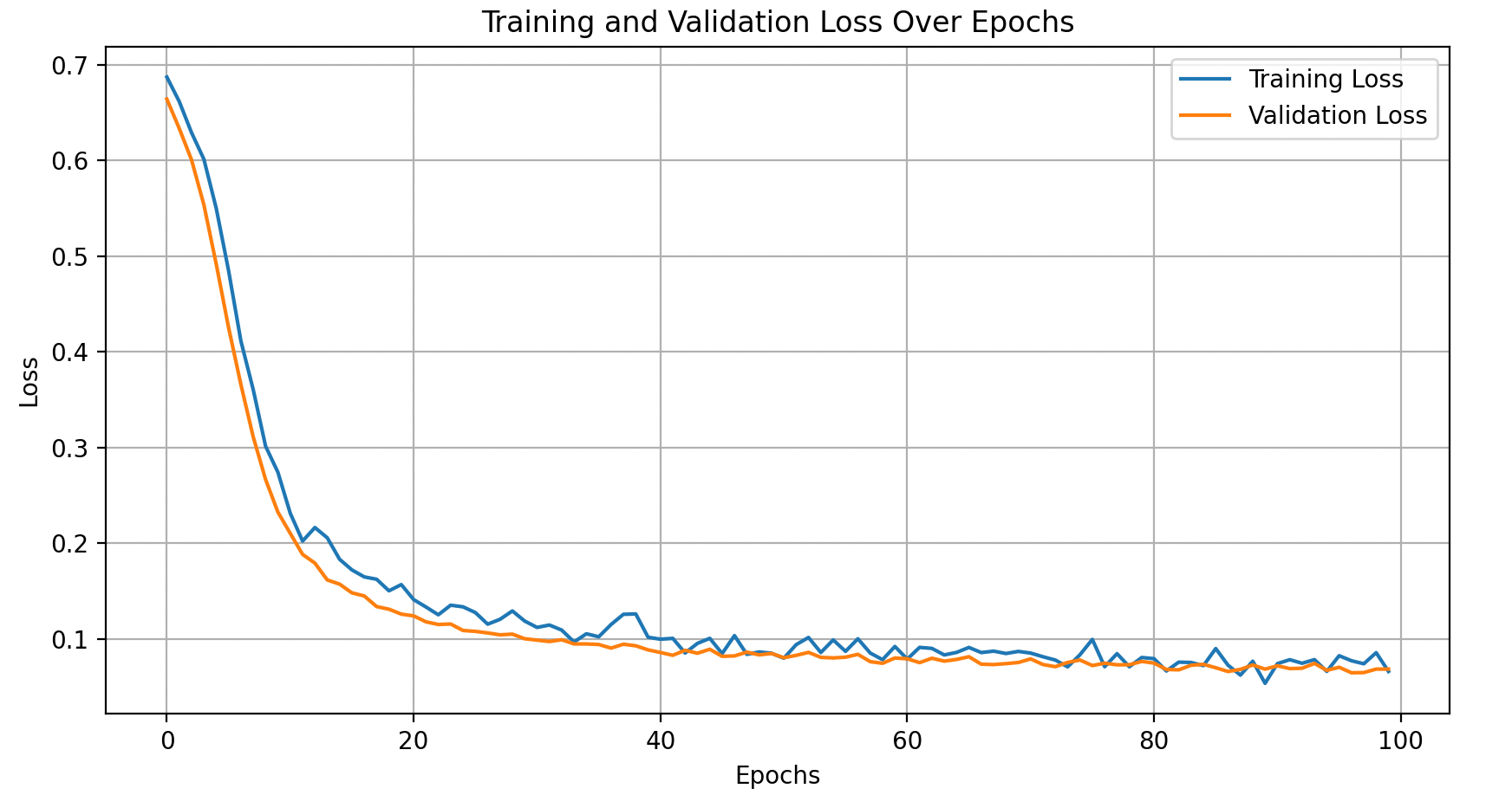
# Train the model
train_losses = train_model(model, train_loader, criterion, optimizer, num_epochs=100)This is what we get we train the model and plot training, validation loss
Evaluating the Model
After training, we need to evaluate our model's performance:
def evaluate_model(model, test_loader, criterion):
    model.eval()  # Set model to evaluation mode
    test_loss = 0.0
    correct = 0
    total = 0

    # No gradient calculation needed for evaluation
    with torch.no_grad():
        for inputs, targets in test_loader:
            # Forward pass
            outputs = model(inputs)

            # Calculate loss
            loss = criterion(outputs, targets)
            test_loss += loss.item() * inputs.size(0)

            # Calculate accuracy
            predicted = (outputs > 0.5).float()
            total += targets.size(0)
            correct += (predicted == targets).sum().item()

    # Calculate metrics
    avg_loss = test_loss / len(test_loader.dataset)
    accuracy = correct / total

    return avg_loss, accuracy

# Evaluate the model
test_loss, test_accuracy = evaluate_model(model, test_loader, criterion)
print(f'Test Loss: {test_loss:.4f}')
print(f'Test Accuracy: {test_accuracy:.4f}')
Visualizing Results
Let's create visualizations to better understand our model:
# Plot training loss
plt.figure(figsize=(10, 5))
plt.plot(train_losses, label='Training Loss')
plt.title('Training Loss Over Epochs')
plt.xlabel('Epochs')
plt.ylabel('Loss')
plt.legend()
plt.grid(True)
plt.show()

# Visualize decision boundary
def plot_decision_boundary(model, X, y):
    # Set min and max values with some margin
    x_min, x_max = X[:, 0].min() - 0.5, X[:, 0].max() + 0.5
    y_min, y_max = X[:, 1].min() - 0.5, X[:, 1].max() + 0.5

    # Create a mesh grid
    h = 0.01  # Step size
    xx, yy = np.meshgrid(np.arange(x_min, x_max, h), np.arange(y_min, y_max, h))

    # Predict for each point in the mesh
    Z = model(torch.FloatTensor(np.c_[xx.ravel(), yy.ravel()])).detach().numpy()
    Z = Z.reshape(xx.shape)

    # Plot the contour and data points
    plt.figure(figsize=(10, 8))
    plt.contourf(xx, yy, Z, cmap=plt.cm.Spectral, alpha=0.8)
    plt.scatter(X[:, 0], X[:, 1], c=y, cmap=plt.cm.Spectral)
    plt.title('Decision Boundary')
    plt.xlabel('Feature 1')
    plt.ylabel('Feature 2')
    plt.show()

# Convert tensors to numpy for plotting
X_all = torch.cat((X_train, X_test), 0).numpy()
y_all = torch.cat((y_train, y_test), 0).numpy().flatten()

# Plot decision boundary
plot_decision_boundary(model, X_all, y_all)
Saving and Loading the Model
To use your trained model later
# Save the model
torch.save(model.state_dict(), 'mlp_model.pth')

# Load the model (for later use)
loaded_model = MLP(input_size, hidden_sizes, output_size)
loaded_model.load_state_dict(torch.load('mlp_model.pth'))
loaded_model.eval()  # Set to evaluation mode
Advanced Techniques for Improving MLP Performance
Learning Rate Scheduling
# Define a learning rate scheduler
scheduler = optim.lr_scheduler.ReduceLROnPlateau(optimizer, 'min', patience=5, factor=0.5)

# Modify training loop to use scheduler
def train_with_scheduler(model, train_loader, criterion, optimizer, scheduler, num_epochs=100):
    # Training code as before
    # ...

    # Add scheduler step after each epoch
    scheduler.step(epoch_loss)

    # ...
Weight Initialization
# Custom weight initialization
def init_weights(m):
    if type(m) == nn.Linear:
        torch.nn.init.xavier_uniform_(m.weight)
        m.bias.data.fill_(0.01)

# Apply to model
model.apply(init_weights)
Early Stopping
def train_with_early_stopping(model, train_loader, val_loader, criterion, optimizer, patience=10, num_epochs=100):
    best_val_loss = float('inf')
    counter = 0

    for epoch in range(num_epochs):
        # Training code as before
        # ...

        # Validation after each epoch
        val_loss, _ = evaluate_model(model, val_loader, criterion)

        # Check if validation loss improved
        if val_loss < best_val_loss:
            best_val_loss = val_loss
            counter = 0
            # Save best model
            torch.save(model.state_dict(), 'best_model.pth')
        else:
            counter += 1

        # Check early stopping condition
        if counter >= patience:
            print(f'Early stopping at epoch {epoch+1}')
            break
Multilayer Perceptrons provide a powerful foundation for understanding neural networks. Through this guide, we've covered setting up, training, evaluating, and improving MLPs using PyTorch. These concepts form the basis for more complex deep learning architectures.