Top Machine Learning Algorithms for Real-World Machine Learning

Linear Regression

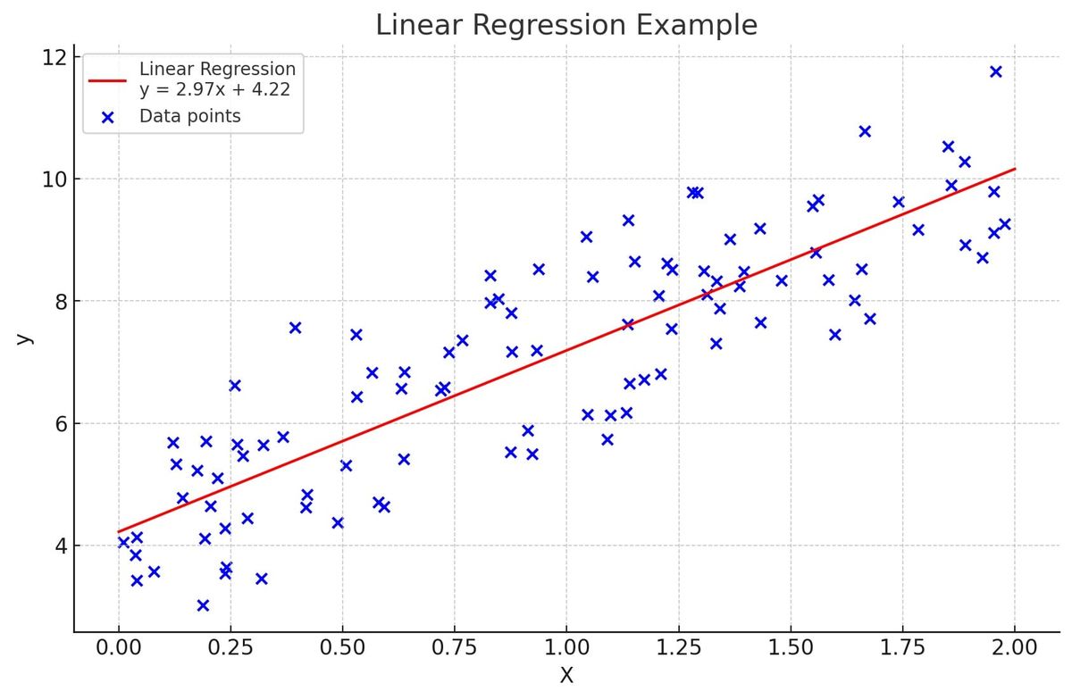
Linear regression is one of the most fundamental and commonly used statistical and machine-learning techniques. At its core, linear regression involves fitting a straight line through a set of data points to be able to make predictions about future data points.

The basic idea behind linear regression is that there is a linear, or straight-line, relationship between the input variables (x) and the output variable (y). The line of best fit is calculated using the least squares method, which minimizes the distance between the observed data points and the line itself.

The linear regression line is described by the equation y=mx+b, where m is the slope of the line and b is the y-intercept - the point where the line crosses the y-axis. Once this line equation is established using existing x and y data points, we can predict the value of y for a new data point by simply plugging its x value into the equation.

Applications of linear regression are extremely widespread, as many real-world relationships demonstrate correlation even if not pure linearity. Examples include predicting housing prices based on square footage, predicting exam scores based on time spent studying, forecasting financial asset performance based on historical returns, and countless more examples. The simplicity and interpretability of linear regression makes it an essential first-pass analysis before exploring more complex machine learning approaches.

By fitting a straight line to data, linear regression allows us to model numerical relationships and make predictions. It lays the foundation for many more sophisticated statistical learning methods used across industries and disciplines. The interpretation of the slope and intercept parameters also provides insight into the relationship between variables. For these reasons, linear regression remains integral to data science and quantitative analysis.

Logistic Regression

Logistic regression[1] is a fundamental statistical and machine learning technique used for modeling the probability of an outcome given one or more input variables. It is a specialized form of regression used when the response variable is categorical, such as true/false or pass/fail.

Whereas linear regression outputs a continuous numeric prediction, logistic regression transforms its output using the logistic sigmoid function to return a probability value constrained between 0 and 1. This probability indicates the likelihood of an observation falling into one of the categories - for example, the probability that an email is spam.

The logistic regression model calculates log-odds as a linear combination of the input variables, then converts the log-odds to probability values using the logistic sigmoid or logistic curve. The familiar linear regression equation is Y=a+bX, while for logistic regression the equation is Log(Odds) = b0 + b1X1 + b2X2 + ..., where the regression coefficients indicate the effect of each variable on the log-odds and consequently on the probability.

Logistic regression does not make any assumptions about the distributions of the input features, allowing for more flexibility compared to methods like linear discriminant analysis. It also does not assume linear relationships between the independent variables and does not require normally distributed error terms. These characteristics make the technique well-suited for binary classification tasks.

Applications of logistic regression are extremely diverse, including medical imaging diagnosis, credit risk assessment, spam email filtering, ecology modeling, gene prediction and more. It is a workhorse method for classification use cases across social sciences, marketing, computer vision, natural language processing, and other realms.

While complex nonlinear machine learning approaches like neural networks have surged in popularity, logistic regression remains vitally important and is often used as a baseline classifier. Its relative simplicity, speed, stability, and ease of interpretation provide practical advantages that often make it the right tool for the job. For binary classification tasks of all kinds, logistic regression should be one of the first methods tried before exploring more exotic options.

Decision Tree

A decision tree is a flowchart-like structure that is used to model decisions and their possible consequences. It is a commonly used machine learning algorithm for both classification and regression predictive modeling problems.

The structure of a decision tree consists of:

• Nodes: Decision nodes and leaves
• Branches: Possible outcomes
• Root node: The starting node

Each decision node represents a test or choice between multiple alternatives. The branches coming out of the decision nodes represent the possible outcomes. At the end of the branches are leaf nodes that represent the final outcomes or decisions.

To build a decision tree, the goal is to identify the input variables that split the dataset into different output categories as much as possible. Common algorithms for building decision trees include ID3, C4.5, and CART.

The ID3 algorithm, developed by Ross Quinlan in 1986, uses information gain as the splitting criterion. Information gain measures how well a given attribute separates the training data according to their target classification. The attribute with the highest information gain is selected as the splitting attribute at each node. The information gain is calculated as:

IG(T,a)=H(T)-H(T|a)

Where:
T = set of training tuples/examples
a = attribute
H(T) = entropy of set T
H(T|a) = entropy of set T given attribute a

C4.5 is a successor of ID3 and removed the bias in information gain when dealing with attributes with a large number of distinct values. CART (Classification and Regression Trees) can build both classification and regression decision trees by using Gini index or Twoing criterion.

The advantages of using decision trees include being easy to interpret and explain, able to handle both numerical and categorical data, uses a white box model, and performs well even if a small dataset is available. Limitations include they can easily overfit, finding the right tree size is a challenge, and small variations in the data can lead to a different tree.

Some additional equations for common tree splitting criteria are:

Gini index:
G(T) = 1 - Σ[P(i|T)]^2

Twoing criterion:
δ(T)=|T1|-|T2|

Where T1 and T2 are the two descendent nodes after splitting

This covers the key aspects of decision trees - their structure, common algorithms, advantages and limitations, and some additional mathematical equations around splitting criteria that can be used. The additional equations help explain some of the underlying math used in constructing decision trees.

SVM (Support Vector Machine)

A support vector machine (SVM) is a supervised machine learning algorithm used for both classification and regression tasks. The goal of an SVM is to create the best separation hyperplane that distinctly classifies the training data points.

The separation hyperplane is the decision boundary that separates data points from different classes. The dimension of the hyperplane depends on the number of features. If the features are two-dimensional, the separation hyperplane will be a line. For higher dimensions, the hyperplane becomes harder to visualize but works in the same way.

An optimal hyperplane maximizes the margin between it and the nearest data points on each side. These closest data points are called the support vectors and directly affect the optimal positioning and orientation of the hyperplane. Finding the maximum margin allows for better generalization and predictive capabilities for unseen data.

To find an optimal hyperplane, SVMs employ an iterative optimization procedure that maximizes the margin while minimizing classification errors. Most SVM algorithms use a kernel trick to transform lower dimension data to higher dimensions to make it possible to find a separation; some common kernels include:

Radial basis function (RBF) kernel:
K(x, x') = exp(-γ ||x - x'||^2)

Polynomial kernel:
K(x, x') = (γx^T x' + c)^d

Where:
γ, c, d are kernel parameters

SVMs can efficiently perform nonlinear classification using what is called the kernel trick, implicitly mapping inputs into high-dimensional feature spaces.

Some major advantages of SVMs include high dimensional space classification, effective in high dimensional spaces, memory efficiency, versatile as different kernel functions can be applied based on the data type. Limitations include being prone to overfitting, requiring careful parameter tuning, and lack of transparency as it uses a black box model.

Additional key SVM equations:

SVM hypothesis function:
f(x) = w^T x + b

Functional margin:
\hat{\rho} = yf(x)

Where:
w = normal vector to hyperplane
b = bias term
y = {-1, +1} target value

This gives an overview of support vector machines, their goal of finding optimal separation hyperplanes, use of kernels, advantages, limitations, and some of the important mathematical equations for understanding how they operate.

Naive Bayes

Naive Bayes is a simple but surprisingly effective statistical classification algorithm used for predictive modeling and making predictions given new data. It is called "naive" because it relies on two very simplifying assumptions about the relationship between the input variables (or features) and the output variable.

First, it assumes that each input variable is independent and does not interact or correlate with any of the others. Second, it assumes that each input variable contributes independently to the probability of a given output. While these assumptions are obviously naive in real-world data, in practice they seem to work quite well in a variety of situations.

The Naive Bayes algorithm uses the joint probabilities of input variables to estimate the conditional probabilities of output categories. By applying Bayes' Theorem, it can calculate the posterior probability of each output given the input data, and the output category with the highest probability is the model's prediction.

Despite its simplicity, Naive Bayes often competes very well with much more complex classifiers and learning algorithms. It scales well to very large datasets since it only requires tabulating the frequencies and conditional probabilities from the training data. Its mathematical foundations are also well understood compared to modern opaque machine learning approaches.

Use cases of Naive Bayes are far-ranging, including text classification, spam filtering, information retrieval, machine learning, data mining and more. It serves as a simple baseline classifier to benchmark against more elaborate methods. Specific applications stretch across subject areas such as biology, psychology, medicine, physics, engineering and computer science.

While it has its weaknesses, Naive Bayes' speed, ease of implementation and transparency offer practical strengths. The volume of data in the real world is growing exponentially, and Naive Bayes has proven that less is often more when tackling complex modeling tasks. Its surprisingly robust performance given its simplicity and limitations has helped it persist as a viable technique worthy of consideration. For these reasons, Naive Bayes retains an important place in the data science toolkit among both well-established and state-of-the-art approaches.

efficiency

Refs